Activity Information
Learning Goals
- Develop a computational model of an RC circuit
- Understand the mathematical relationships between I,Q, and V in an RC circuit
- Compare numerical and analytical solutions
Prior Knowledge Required
- Ohm’s Law
- Q = CV
- Kirchhoff’s Loop Rule for Voltage
- I = dQ/dt
Code Manipulation
- Create code from mathematical equations
- Copy/Paste code
Activity
Handout – Celestial Circuitry
Part 1
You and your friends are out for a lovely evening bike ride when you happen upon the deserted wreck of an alien spacecraft. Curious to see what secrets it contains, you take a look inside, but the ship’s door slams shut once you are all inside.
You investigate the spaceship and find this program on its computer along with the following note:
Pilot's Starlog 10878.5
Ship power is down. I think an emergency battery could be used to restart the main reactor by using it to charge a capacitor in an RC circuit. The battery is 10 V, the capacitor is 0.1 F and I have 3 resistors to choose from, which are 5,10, and 20 Ω respectively. I'll need to be careful - if ≥ 1 A is drawn from the battery at any point, it could explode.

To make sure the circuit works flawlessly, I've created a code to simulate and visualize the charging circuit. Hopefully I can finish it before the ship crashes....
For you to escape the ship, you’ll need to finish the Pilot’s code. You can move on to part 2 once you finish the code for part 1. Good luck!
Part 2
As you finish your code, you find another note from the pilot:
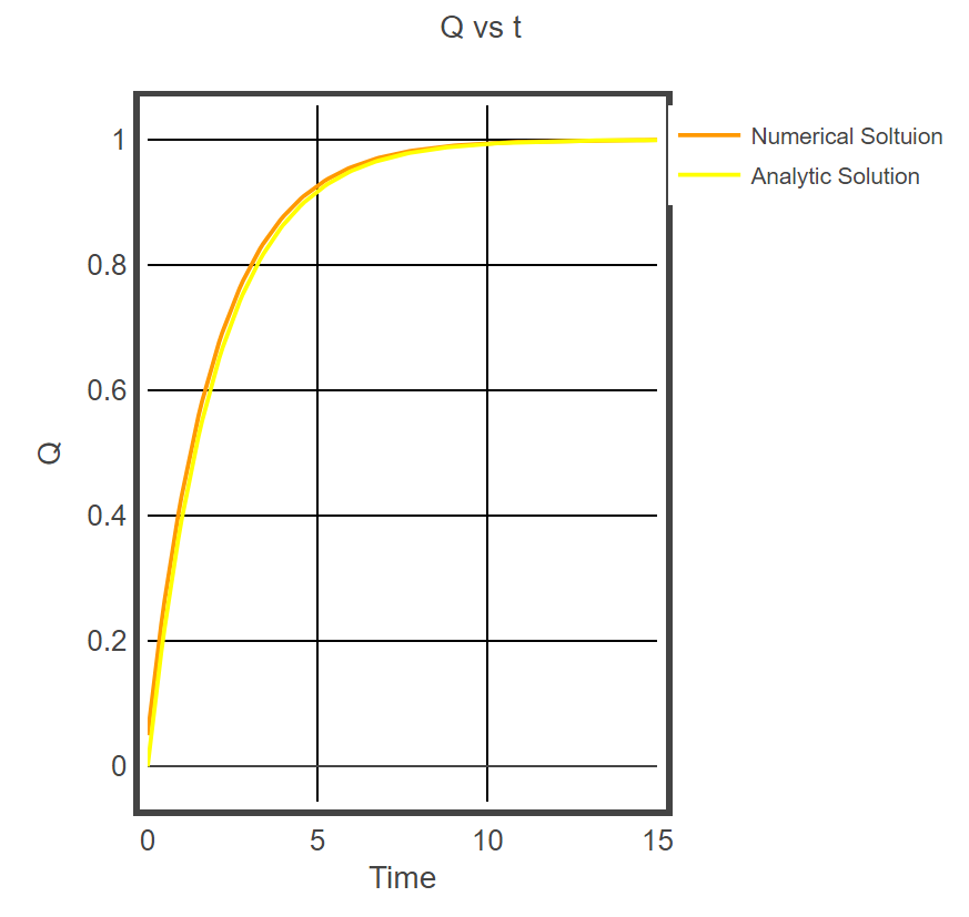
Pilot's Starlog 10878.8
I've found the analytical solution to the charge in the circuit! It is:
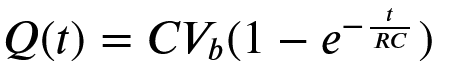
I wonder if this will be close to the computer's numerical solution....
Add this solution to your code and graph it alongside the solution you’ve already coded. Hint: e^x in glowscript is exp(x).
Post-Coding Questions:
- Which resistor did you choose? Why?
- When is the maximum current drawn from the battery?
- How can you make the numerical solution more accurate?
- What Assumptions did you make when solving this problem?
- After a very long time, what are the values for Q, V, and I? Answer in variables for Q and V.
Code
GlowScript 3.1 VPython
scene.background = color.white
#Object setup
wire1 = cylinder(pos = vec(-0.5,-0.5,0), axis = vec(1,0,0),radius = 0.01,color = color.black)
wire2 = cylinder(pos = vec(-0.5,0.5,0), axis = vec(0.48,0,0),radius = 0.01,color = color.black)
wire3 = cylinder(pos = vec(0.5,0.5,0), axis = vec(-0.48,0,0),radius = 0.01,color = color.black)
wire4 = cylinder(pos = vec(-0.5,-0.5,0), axis = vec(0,1,0),radius = 0.01,color = color.black)
wire5 = cylinder(pos = vec(0.5,-0.5,0), axis = vec(0,1,0),radius = 0.01,color = color.black)
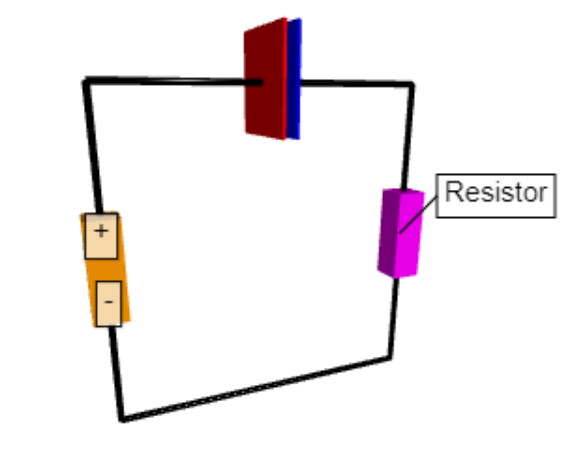
capacitorplate1 = box(pos = vec(-0.02,0.5,0),size = vec(0.01,0.3,0.3),color = color.black)
capacitorplate2 = box(pos = vec(0.02,0.5,0),size = vec(0.01,0.3,0.3),color = color.black)
battery = box(pos = vec(-0.5,0,0),size = vec(0.1,0.3,0.1), color = color.orange)
resistor = box(pos = vec(0.5,0,0),size = vec(0.1,0.3,0.1),color = color.magenta)
label1 = label(pos=vec(-0.5,0.1,0),text='+', height=16, border=4,font='sans')
label2 = label(pos=vec(-0.5,-0.1,0),text='-', height=16, border=4,font='sans')
label3 = label(pos=vec(0.5,0,0),text='Resistor', xoffset = 20,yoffset = 20,height=15, border=4,font='sans')
#model parameters
Vbatt = 10 # Volts
R =
Q = 0 # coulombs
C = # Farads
#time setup
t = 0
tf = 10
dt = 0.1
#graph setup
Qgraph = graph(title='Q vs t', xtitle='Time', ytitle = 'Q', fast=False, width=480)
f1 = gcurve(color=color.orange, label = 'Numerical Soltuion')
Vgraph = graph(title='Vc vs t', xtitle='Time', ytitle = 'V', fast=False, width=480)
f2 = gcurve(color=color.red)
Igraph = graph(title='I vs t', xtitle='Time', ytitle = 'I', fast=False, width=480)
f3 = gcurve(color=color.orange)
#click to run
print("Click the program window to run.")
ev = scene.waitfor('click')
#loop to make things happen
while t<tf:
rate(100)
I = 0 # Hint: Use a loop rule
Q = Q # Hint: I = dQ/dt
Vc = 0 # calculate the voltage
# plot stuff
f1.plot(t,Q)
f2.plot(t,Vc)
f3.plot(t,I)
# The next two lines update the color of the capacitor plates as it charges
# + plate should turn red, - plate should turn blue
capacitorplate1.color = vec(Q/(C*Vbatt),0,0)
capacitorplate2.color = vec(0,0,Q/(C*Vbatt))
t = t + dt # increment the timeAnswer Key
Handout
First let’s add the correct values in lines 18-22:
#model parameters
Vbatt = 10  # Volts
R = 20      # ohms
Q = 0       # coulombs
C = 0.1     # Farads
We’ll discuss why the 20 Ω resistor was chosen in post-coding question 1.
Next, we’ll need to find an equation for I to input in line 45. To do this we can use Kirchhoff’s loop rule for the circuit. There’s only one loop here so we don’t need to worry about choosing an appropriate loop. Let’s loop around the circuit clockwise, starting from the battery:
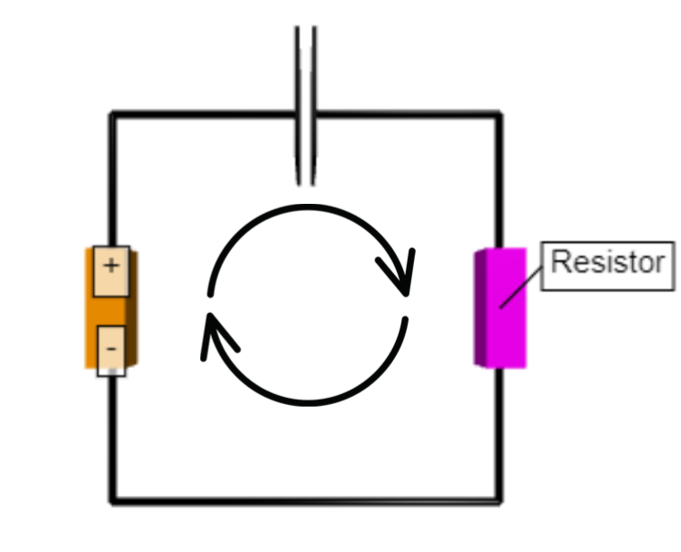
This gives us the equation:
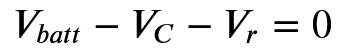
Where Vc is the voltage drop across the capacitor and Vr is the voltage drop across the resistor. We can then use V = IR and Q = CV to write this equation as:
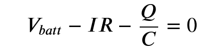
Which can then be rearranged to:
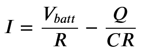
Adding this to the code looks like:
I = Vbatt/R - Q/(C*R)Recalling that I = dQ/dt, we can use I to update Q in the next line:
Q = Q + I*dt We can use V = Q/C in the next line to calculate the voltage drop across the resistor Vc:
Vc = Q/C This completes part 1.
To add the analytical solution to the code, we can simply add another line beneath the line that calculates the voltage across the capacitor:
Qanalytic = C*Vbatt*(1-exp(-t/(R*C)))To graph this, we can duplicate line 31 and modify it slightly so it is appropriate for the analytic solution:
f4 = gcurve(color=color.yellow, label = 'Analytic Solution')We’ll have to add another line in the while loop to actually plot this solution as well:
f4.plot(t,Qanalytic)This concludes the coding portion of the problem.
Post-Coding Questions:
- We chose the 20 Ω resistor because the maximum current drawn from the battery is too large with the 5 Ω and 10 Ω resistors. We can find the max current by using Ohm’s law solved for I: I = V/R and plugging in Vbatt for V and the 3 resistances for R. We can do this because capacitors act like wires initially. This gives us the following results:
| R (Ω) | Imax (A) |
| 5 | 2 |
| 10 | 1 |
| 20 | 0.5 |
2. Imax occurs at t = 0.
3. We can make the numerical solution more accurate by making dt smaller.
4. We assumed that the wires had no resistance and that the battery had no internal resistance.
5. After a long time, Vc = Vbatt and I = 0. This is because capacitors act like open switches after a long time. When the capacitor acts like an open switch, then no current can flow and then the loop equation tells us that Vc = Vbatt. We can then use this voltage to see that Q = CVbatt.
Code
GlowScript 3.1 VPython
scene.background = color.white

#Object setup
wire1 = cylinder(pos = vec(-0.5,-0.5,0), axis = vec(1,0,0),radius = 0.01,color = color.black)
wire2 = cylinder(pos = vec(-0.5,0.5,0), axis = vec(0.48,0,0),radius = 0.01,color = color.black)
wire3 = cylinder(pos = vec(0.5,0.5,0), axis = vec(-0.48,0,0),radius = 0.01,color = color.black)
wire4 = cylinder(pos = vec(-0.5,-0.5,0), axis = vec(0,1,0),radius = 0.01,color = color.black)
wire5 = cylinder(pos = vec(0.5,-0.5,0), axis = vec(0,1,0),radius = 0.01,color = color.black)
capacitorplate1 = box(pos = vec(-0.02,0.5,0),size = vec(0.01,0.3,0.3),color = color.black)
capacitorplate2 = box(pos = vec(0.02,0.5,0),size = vec(0.01,0.3,0.3),color = color.black)
battery = box(pos = vec(-0.5,0,0),size = vec(0.1,0.3,0.1), color = color.orange)
resistor = box(pos = vec(0.5,0,0),size = vec(0.1,0.3,0.1),color = color.magenta)
label1 = label(pos=vec(-0.5,0.1,0),text='+', height=16, border=4,font='sans')
label2 = label(pos=vec(-0.5,-0.1,0),text='-', height=16, border=4,font='sans')
label3 = label(pos=vec(0.5,0,0),text='Resistor', xoffset = 20,yoffset = 20,height=15, border=4,font='sans')

#model parameters
Vbatt = 10  # Volts
R = 20      # ohms
Q = 0       # coulombs
C = 0.1     # Farads

#time setup
t = 0
tf = 15
dt = 0.1

#graph setup
Qgraph = graph(title='Q vs t', xtitle='Time', ytitle = 'Q', fast=False, width=480)
f1 = gcurve(color=color.orange, label = 'Numerical Soltuion')
f4 = gcurve(color=color.yellow, label = 'Analytic Solution')
Vgraph = graph(title='Vc vs t', xtitle='Time', ytitle = 'V', fast=False, width=480)
f2 = gcurve(color=color.red)
Igraph = graph(title='I vs t', xtitle='Time', ytitle = 'I', fast=False, width=480)
f3 = gcurve(color=color.orange)

#click to run
print("Click the program window to run.")
ev = scene.waitfor('click')

#loop to make things happen
while t<tf:
  rate(100)

  I = Vbatt/R - Q/(C*R) # find the instantaneous change in Q
  Q = Q + I*dt          # update Q
  Vc = Q/C              # calculate the voltage
  Qanalytic = C*Vbatt*(1-exp(-t/(R*C)))

  # plot stuff, update colors
  f1.plot(t,Q)
  f2.plot(t,Vc)
  f3.plot(t,I)
  f4.plot(t,Qanalytic)
  capacitorplate1.color = vec(Q/(C*Vbatt),0,0)
  capacitorplate2.color = vec(0,0,Q/(C*Vbatt))

  t = t + dt # increment the time