Activity Information
Learning Goals
- Develop a computational model to visualize an electromagnetic wave
- Understand how nested loops work
Prior Knowledge Required
- Vectors
- Electromagnetic wave equations
- E = E0 sin(kx – ωt)
- B = B0 sin(kx – ωt)
- How f, ω, λ, and c relate to each other in light waves
- E/B = c
Code Manipulation
- Interpret existing code
- Create new code from mathematical equations
Activity
Handout – Electromagnetic Investigation
You and your elite team of super-spies, the Proficient Espionage and Reconnaissance Lineup (P.E.R.L.), have decided to investigate the strange disappearance of Meghanne Quartz, your team’s scientist.
You remember that Quartz is a member of the secretive but scientific organization the League of Meticulous Analytics and Observations (L.M.A.O.) so you contact them, asking for any information they may have. You quickly receive a reply:
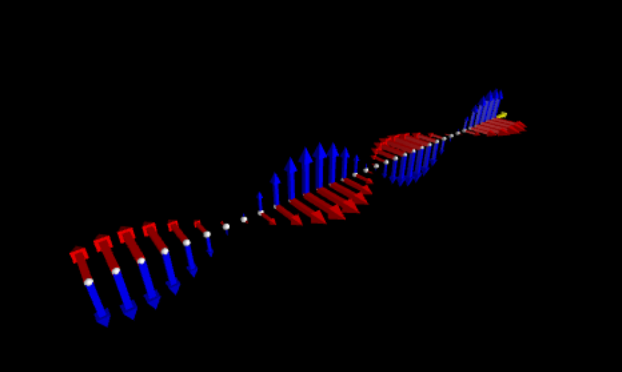
We do have information pertaining to the disappearance of Ms. Quartz. However, for us to share that information, you must prove to us that you are true supporter of science.

If you are able to accurately complete this program, which is a simulation of an electromagnetic wave with λ = 4 m and Bmax = 1*10^-7 T, we will share the aforementioned information.
You and your team will have to use your physics and coding skills to complete the code and obtain the clue. Good luck!
Optional bonus challenge:
Add a Poynting vector for the observation point furthest to the right.
Code
GlowScript 3.1 VPython

scene.range = 3.8

obs = vec(-5,0,0) # Initial observation location
dx = 0.3
Elist = []
Blist = []

while obs.x <= 5:
  dot = sphere(pos=obs, radius = 0.05) # Place a dot at each observation point
  Earrow = arrow(pos=obs, axis = vec(0,0,0), color = color.blue) # place an E-field arrow at each observation point
  Elist.append(Earrow) # Store all of the E-Field arrows in a list
  Barrow = arrow(pos=obs, axis = vec(0,0,0), color = color.red) # place a B-Field arrow at each observation point
  Blist.append(Barrow) # Store all of the B-Field arrows in a list

  obs.x = obs.x + dx # Increment in the x direction

# Constants setup
wavelength = 6 # m
c = 3e8        # m/s
k = (2*pi)/wavelength
w = 0 # should not be zeros
B0 = 0
E0 = 0

# Scaling Setup - should not be zeros
Escale = 0
Bscale = 0

# Time setup
t = 0
tf = 5e-8
dt = 1e-10

#click to run
print("Click the program window to run.")
ev = scene.waitfor('click')

# loops to make things happen
while t<tf:
  rate(80)
  for E in Elist:
    E.axis = vec(0,1,0)

  for B in Blist:
    B.axis = vec(0,0,1)


  t = t + dt
Answer Key
Handout
answer key
First, let’s calculate the correct values for w, BO, and E0 in lines 23, 24, and 25, respectively.
For w, which is really representing ω, we can start with the equation
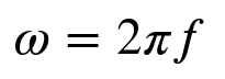
and then use:
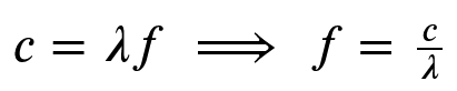
To get an equation for ω in terms of variables that are known:
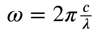
In the code, this looks like:
w = 2*pi*c/wavelength # rad/sNext, B0 is given in the problem statement as Bmax = 1*10^-7 T. which is easy to enter into code:
B0 = 1e-7 # TTo find E0, we can use the fact that E/B = c => Bc = E:
E0 = B0*c # V/mWe’ll skip the scaling factors for now and go straight to the loops. To change these loops so that they represent the correct values, we can simply change the 1s in lines 44 and 47 to the electromagnetic wave equations:
in the code this looks like:
while t<tf:
  rate(80)
  for E in Elist:
    E.axis = vec(0,E0*sin(k*E.pos.x -w*t),0)

  for B in Blist:
    B.axis = vec(0,0,B0*sin(k*B.pos.x -w*t))

  t = t + dt
Now we can to experiment to find the right scaling factors to make the waves look nice, the following values work quite well:
# Scaling Setup
Escale = 3e-2
Bscale = 1e7
We can then use these values in the loops:
while t<tf:
  rate(80)
  for E in Elist:
    E.axis = Escale*vec(0,E0*sin(k*E.pos.x -w*t),0)

  for B in Blist:
    B.axis = Bscale*vec(0,0,B0*sin(k*B.pos.x -w*t))

  t = t + dt
Bonus Challenge Solution
To add a Poynting vector, we will first initialize it anywhere before the nested loops:
# Initialize Poynting Vector
P = arrow(pos=vec(5,0,0), axis = vec(0,0,0), color = color.yellow)
We’ll also need to add a new scaling factor and the value of μ0 to the code before the nested loops:
mu0 = 4*pi*10e-7

Pscale = 4*pi*10e-7
Finally, we can use the glowscript cross function to update the axis of the Poynting vector:
# While loop to make things happen
while t<tf:
  rate(80)
  for E in Elist:
    E.axis = Escale*vec(0,E0*sin(k*E.pos.x -w*t),0)

  for B in Blist:
    B.axis = Bscale*vec(0,0,B0*sin(k*B.pos.x -w*t))

  P.axis = (Pscale/mu0)*cross(E.axis,B.axis) # Update Poynting vector

  t = t + dt
Code
GlowScript 3.1 VPython

scene.range = 3.8

obs = vec(-5,0,0) # Initial observation location
dx = 0.3
Elist = []
Blist = []

# Initialize Poynting Vector
P = arrow(pos=vec(5,0,0), axis = vec(0,0,0), color = color.yellow)

while obs.x <= 5:
  dot = sphere(pos=obs, radius = 0.05) # Place a dot at each observation point
  Earrow = arrow(pos=obs, axis = vec(0,0,0), color = color.blue) # place an E-field arrow at each observation point
  Elist.append(Earrow) # Store all of the E-Field arrows in a list
  Barrow = arrow(pos=obs, axis = vec(0,0,0), color = color.red) # place a B-Field arrow at each observation point
  Blist.append(Barrow) # Store all of the B-Field arrows in a list

  obs.x = obs.x + dx # Increment in the x direction

# Constants setup
wavelength = 6 # m
c = 3e8        # m/s
k = (2*pi)/wavelength
w = 2*pi*c/wavelength # rad/s
B0 = 1e-7 # T
E0 = B0*c # V/m
mu0 = 4*pi*10e-7

# Scaling Setup
Escale = 3e-2
Bscale = 1e7
Pscale = 4*pi*10e-7

# Time setup
t = 0
tf = 5e-8
dt = 1e-10

#click to run
print("Click the program window to run.")
ev = scene.waitfor('click')

# While loop to make things happen
while t<tf:
  rate(80)
  for E in Elist:
    E.axis = Escale*vec(0,E0*sin(k*E.pos.x -w*t),0)

  for B in Blist:
    B.axis = Bscale*vec(0,0,B0*sin(k*B.pos.x -w*t))

  P.axis = (Pscale/mu0)*cross(E.axis,B.axis) # Update Poynting vector

  t = t + dt