Recursive Modeling with Acceleration – Integrating Computation in Science Across Michigan

Activity Information

Learning Goals

Interpret a computational model of an accelerating object
Analize data to identify the relationships between position, velocity, and acceleration (HS-PS2-1)

Prior Knowledge Required

Vectors
1D Kinematics

Code Manipulation

Interpret existing code

Activity

Handout – Recursive Modeling with Acceleration

A computer creates the illusion of movement by drawing an object over and over in slightly different positions each time. If the displacement between positions is small enough and the computer does it quickly enough, the motion will look smooth and natural.

The type of motion is determined by whoever creates the model, depending on what they are trying to recreate. To have the computer show an object undergoing constant acceleration, you can create an approximate model of the position of the object over time using constant velocity for short segments of time and calculating the next position using the most recent values for velocity and position.

Consider this code:

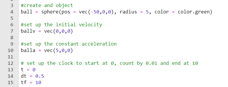
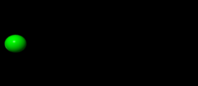
1. What kind of object will the computer show?

2. What is the object’s initial position?

3. What is the object’s initial velocity?

4. What acceleration is the object experiencing?

5. What is the starting time?

6. What time interval does the clock count by?

Now consider this part of the code:

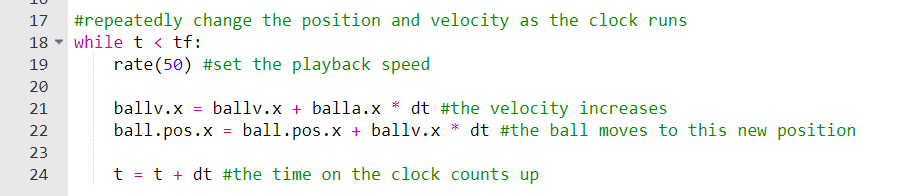
7. When will the while-loop stop running? Be specific.

The computer follows the instructions in the while-loop step by step. You are going to execute the commands as the computer would and fill in the table below. Note that when the computer sees a variable (ball.pos, ballv or t) followed by an equal sign, it does not fill the known value in for that variable. Instead, it stores whatever value or calculated value that comes after the equal sign as that variable.

For example, when the computer sees

ball.pos.x = ball.pos.x + ballv.x * dt

It calculates the value of −50+0∗0.5, and stores −50 as the new value for ball.pos.x, which is what it will use the next time a calculation involving ball.pos.x is made. The computer does not remember older values for a variable, only the most recent one.

8. Follow the commands in the while-loop to find the values of t, ball.pos.x and ballv.x and fill in this table.

Execution of the while-loop	t	ball.pos.x	ballv.x
0th
1st
2nd
3rd
4th
5th

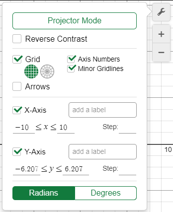
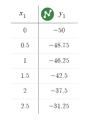
9. Create a table of values in Desmos using t and ball.pos.x. You may need to adjust the scale of the x- and y-axes using the settings. (See below.)

10. Connect the points with straight line segments. What shape does the graph remind you of?

11. What do you think would happen to the graph if the time interval that the clock counts by was much shorter?

12. Why is it necessary to update the velocity value each time?

13. Run this code in Trinket. Does it behave like you expect? Try modifying the code to get the motion to look different. You’ll have to click “remix” to save your own copy.

Code

Link

GlowScript 3.1 VPython



#create and object
ball = sphere(pos = vec(-50,0,0), radius = 5, color = color.green)

#set up the initial velocity
ballv = vec(0,0,0)

#set up the constant acceleration
balla = vec(5,0,0)

# set up the clock to start at 0, count by 0.01 and end at 10
t = 0
dt = 0.5
tf = 10

#repeatedly change the position and velocity as the clock runs
while t < tf:
    rate(100) #set the playback speed
    
    ball.pos.x = ball.pos.x + ballv.x * dt #the ball moves to this new position
    ballv.x = ballv.x + balla.x * dt #the velocity increases
    
    t = t + dt #the time on the clock counts up

Answer Key

Handout

1. A sphere

2. <-50 , 0 , 0> m

3. <0 , 0 , 0> m/s

4. <5, 0 , 0> m/s^2

5. 0 s

6. dt = .5

7. The while loop will stop running when its condition statement “t < tf” is no longer true. This means when the value of t exceeds the specified final time tf, the loop will stop.

8. To fill out this table, go line by line like the python interpreter does. The 0th loop is the initial values. For the first execution of the loop, first update the ball’s velocity according to:

ballv.x = ballv.x + balla.x

Now update its position according to:

ball.pos.x = ball.pos.x + ballv.x * dt

And finally update the time according to:

t = t + dt

Execution of the while-loop	t	ball.pos.x	ballv.x
0th	0	-50	0
1st	0.5	-48.75	2.5
2nd	1	-46.25	5
3rd	1.5	-42.5	7.5
4th	2	-37.5	10
5th	2.5	-31.25	12.5

10. The graph should look something like this:

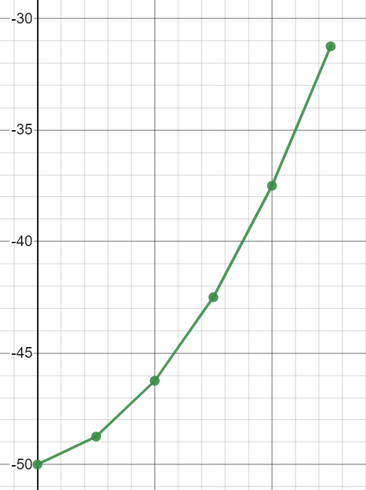
The shape looks like a parabola.

11. If the time interval was smaller, there would be more data points and the graph would look smoother

12. It’s important to update the velocity value each time because the sphere is undergoing constant acceleration, which means that its velocity is always changing.

13. It runs quickly but the motion is as expected. Answers will vary for code modifications.