Visualizing Electric Potential

Activity Information

Learning Goals

• Develop a computational model which represents the electric potential from a point charge

Prior Knowledge Required

• Equation for the voltage from a point charge
• Vector vs Scalar quantities

Code Manipulation

• Edit existing code
• Interpret existing code
• Create code from mathematical equations
• Copy / Paste code

Activity

Handout – Visualizing Electric Potential

The year is 2350. You’re a member of the space-navy of the United Nations of Earth (the UNN), and you’ve recently been promoted to the science team of the UNN Agatha King, a formidable dreadnought.

On its way to investigate a distress beacon near Jupiter, the Agatha King has run into a technical problem: The ships’ sensors have failed! These sensors are critical to the ship being able to navigate safely in space and will need to be repaired quickly.

One of the key sensors operates by detecting fluctuations in the electric potential near a point charge. Upon inspection, you find out that the code that creates a representation of the voltage around the point charge has been tampered with. To get the ship’s sensors back online, you’ll need to fix this broken code.

Post-Coding Questions:

1. Why can we represent the potential from the point charge with only one variable, r, instead of 3 variables: x, y, and z?
2. Why couldn’t we start at r = 0?
3. How could you increase the “smoothness” of the color gradient produced by the program?
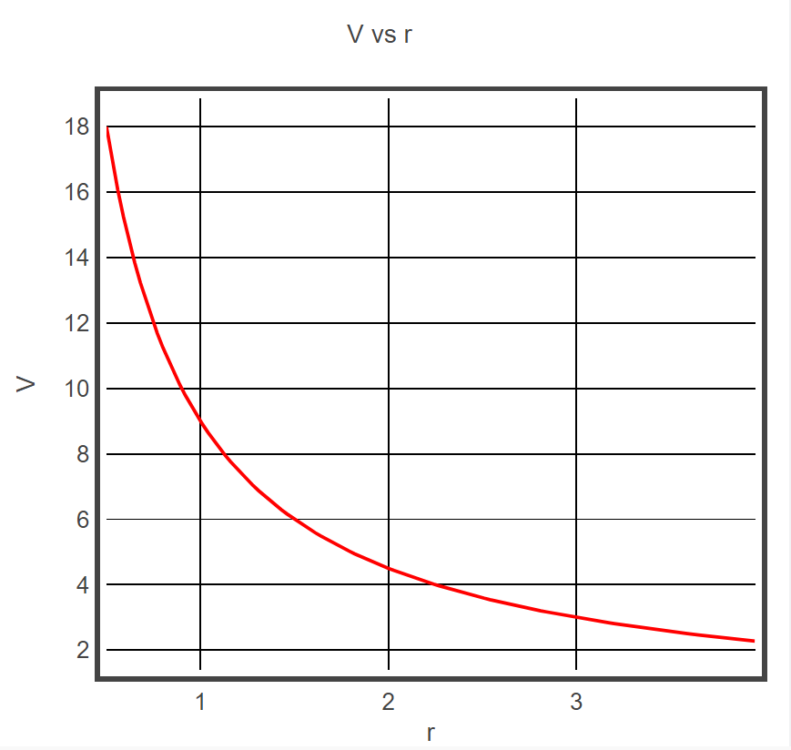
4. As r increases, what value does V approach? Why?

Code

Link

GlowScript 3.1 VPython

# View Setup
scene.range = 1.5
scene.background = color.white

# Object setup
p = sphere(pos = vec(0,0,0),radius = 0.2, color = color.red,q = 1)  # These are the point particles that are creating the E field

# lets define some useful constants
k = 9e9        # Coulomb Constant
r = 0.5        # Initial radius of the first ring
dr = 0.03

# Need equation for V0
V0 = 0 # Initial voltage at the first ring, can be thought of as the max voltage because it will be the closest measurement to the point charge

# Create V vs r graph
Vgraph = graph(title='V vs r', xtitle='r', ytitle = 'V', fast=False, width=480)
f1 = gcurve(color=color.red)

# Place the first ring
ring1 = ring(pos=p.pos,axis=vec(0,0,1), radius=r, thickness=0.1,color = vec(1,0,0)) 

# While loop to place many more rings, with color corrresponding to voltage
while r <= 4: # Run this loop until r is 4
  rate(100)   # rate statement can make it easier to see what the code is doing but is not neccecary
  
  f1.plot(r,V)
  
  r = r + dr

Answer Key

Handout

First, let’s add an equation for V0. We’ll use the equation for the electric potential from a point charge:

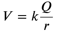
In the code, this looks like:

V0 = (k*p.q)/r

Now we can take a look at the while loop itself. We can use the same equation from above to calculate the voltage at each value of r:

while r <= 4: # Run this loop until r is 4
  rate(100)
  V = (k*p.q)/r
  f1.plot(r,V)
  r = r + dr              

This finishes the V vs R graph below, but we still need to add a new ring at each value of r. We can start doing this by copying the code from line 23 into our while loop:

while r <= 4: # Run this loop until r is 4
  rate(100)
  V = (k*p.q)/r
  f1.plot(r,V)
  ring1 = ring(pos=p.pos,axis=vec(0,0,1), radius=r, thickness=0.1,color = vec(1,0,0))
  r = r + dr 

Let’s change the name from ring1 to something else, because it doesn’t make much sense to call all the rings ring1:

while r <= 4: # Run this loop until r is 4
  rate(100)
  V = (k*p.q)/r
  f1.plot(r,V)
  obsring = ring(pos=p.pos,axis=vec(0,0,1), radius=r, thickness=0.1,color = vec(1,0,0))
  r = r + dr 

Unfortunately, this results in all the rings having the same color, so we will need to change that part of the code for each obsring. Noting that the max value that we can have for any component in the color vector is 1, and our max value of V is V0, we can write:

color = vec(V/V0,0,0)

Which gives us a final while loop that looks like:

# While loop to place many more rings 
while r <= 4: # Run this loop until r is 4
  rate(100)
  V = (k*p.q)/r
  f1.plot(r,V)
  obsring = ring(pos=p.pos,axis=vector(0,0,1), radius=r, thickness=0.1,color = vec(V/V0,0,0))  
  r = r + dr

Post – Coding Questions:

1. We only need one variable r because the electric potential depends only on the relative distance from the observer and the point charge.

2. If we tried to start at r = 0, we would end up dividing by zero, which is undefined.

3. We could decrease the value of dr, which would result in more rings being placed.

4. As r increases, V goes to zero. This is because dividing by a larger number results in a smaller number.

Code

Link

GlowScript 3.1 VPython

# View Setup
scene.range = 1.5
scene.background = color.white

# Object setup
p = sphere(pos = vec(0,0,0),radius = 0.2, color = color.red, q = 1e-9)  # These are the point particles that are creating the E field

# lets define some useful constants
k = 9e9        # Coulomb Constant
r = 0.5        # Initial radius of the first ring
dr = 0.03


V0 = (k*p.q)/r # Initial voltage at the first ring, can be thought of as the max voltage because it will be the closest measurement to the point charge

# Create V vs r graph
Vgraph = graph(title='V vs r', xtitle='r', ytitle = 'V', fast=False, width=480)
f1 = gcurve(color=color.red)

# Place the first ring
ring1 = ring(pos=p.pos,axis=vec(0,0,1), radius=r, thickness=0.1,color = vec(1,0,0))

# While loop to place many more rings 
while r <= 4: # Run this loop until r is 4
  rate(100)
  V = (k*p.q)/r
  f1.plot(r,V)
  obsring = ring(pos=p.pos,axis=vector(0,0,1), radius=r, thickness=0.1,color = vec(V/V0,0,0))  
  r = r + dr