Activity Information
Learning Goals
- Develop a computational model to understand and visualize the relationships between magnetic flux, the change in magnetic flux, and the induced EMF
- Compare Numerical and Analytical solutions to a problem
Prior Knowledge Required
- Vectors
- Trig functions and their derivatives
- How to find flux from a constant field and area
- Φ = BAcos(θ) equation
- Faraday’s law equation
Code Manipulation
- Interpret existing code
- Create new code from mathematical equations
Activity
Handout – EMF Espionage
You and your elite team of super-spies, the Proficient Espionage and Reconnaissance Lineup (P.E.R.L.), have been tasked with infiltrating the secret headquarters of DreadCo, a company that surprisingly few people have realized is evil.
To infiltrate the building, you’ll need to cut through its steel wall with your handy dandy laser cutter. Unfortunately, DreadCo’s security system can detect batteries, so you’ll have to find another way to power it.
However, there is a 1 mT magnetic field emanating from the building. Your team’s scientist Meghanne Quartz thinks that you can use this field with a rotating coil of wire to produce an alternating current capable of powering the laser cutter. To ensure your team’s safety, Quartz created a simulation of the proposed device, but she mysteriously disappeared before finishing it. Thankfully she left behind lots of comments in her code.
It’s up to you and your team to complete the simulation to ensure your safety. Good luck!
Post-Coding Questions:
- How could you increase the induced EMF?
- How could you decrease the numerical error?
- What direction does the induced EMF point? When does it change?
- What assumptions did you make when solving this problem?
Code
GlowScript 3.1 VPython
scene.range = 1.5
# Magnetic field points DOWNWARD
# Objects
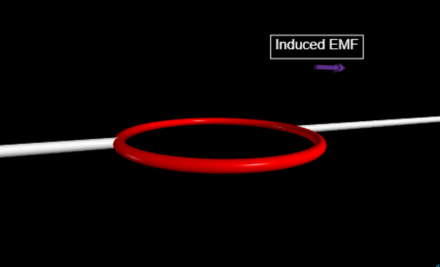
coil = ring(pos=vector(0,0,0), axis=vector(0,1,0), radius=1, thickness=0.05,color = color.red)
wire1 = cylinder(pos=vector(-coil.radius,0,0),radius = coil.thickness,axis = vec(-50,0,0))
wire2 = cylinder(pos=vector(coil.radius,0,0),radius = coil.thickness,axis = vec(50,0,0))
Vindlabel = label(pos=vec(1.25,1,0), text='Induced EMF')
Varrow = arrow(pos = vec(1.25,0.75,0),axis = vec(0,0,0),color = color.purple)
# Graph setup - ignore
Fluxgraph = graph(title='Flux and Change in Flux', xtitle='Time', fast=False, width=500)
f1 = gcurve(color=color.blue, label = 'phi')
f2 = gcurve(color=color.orange,label = 'd phi/dt')
f3 = gcurve(color=color.black, label = "delta phi")
EMFgraph = graph(title='EMF vs t', xtitle='Time', ytitle = 'EMF [V]', fast=False, width=500)
f4 = gcurve(color=color.red, label = "EMF")
Errorgraph = graph(title='Numerical Error', xtitle='Time',ytitle = 'Error', fast=False, width=500)
f5 = gcurve(color=color.blue, label='Error')
# Setting up variables
omega = pi # In rad/s, this means the loop will rotate 180 degrees every second
B=1E-3 # The magnetic field, in Tesla
A = pi*(coil.radius**2) # Area of the loop
N = 500 # Number of loops of wire in the coil
#time setup
t=0
tf = 5
dt = 0.01
#Loop to make stuff happen
while t < tf:
rate(100)
coil.rotate(angle=(omega)*dt, axis=vector(1,0,0), origin=coil.pos) # Rotates the coil
# Not sure what to do with these four lines
# Need a peak EMF of at least 4V to be safe
phi = cos(0) # Should be true value for the Magnetic Flux
deltaphi = 0 # Should be approximate value of dphidt
dphidt = 0 # Should be the true value of dphidt
EMF = 0 # Not sure what relates EMF and dphi/dt
error = abs(dphidt-deltaphi) # Calculate the error of the approximate value of dphi/dt
Varrow.axis = vec(EMF,0,0) #update the Vind arrow's size and direction
f1.plot(t,phi) # Plot everything
f2.plot(t,dphidt)
f3.plot(t,deltaphi)
f4.plot(t,EMF)
f5.plot(t,error)
t = t + dt # Increment the timeAnswer Key
Handout
To complete the code, only lines 41-44 need to be changed. We will discuss each line separatley:
Line 41 -Flux
This line will calculate the flux at each time step. Magnetic flux, or the amount of magnetic field passing through an area is given by:
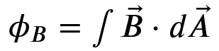
Which can be simplified to :
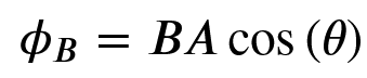
When we have a constant B-Field and Area. θ is the angle between B and dA. The vector rules and calculus to do this simplification are beyond the scope of most high school physics courses so students should be given this equation.
If we choose dA to point downward, then the initial angle between B and dA is 0, so we can use this equation as it is for the flux through one loop.
To get the total flux through the coil, we need to multiply this equation by the number of loops, N:
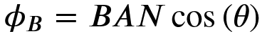
To translate this equation into code, we can use the equation θ = ωt because ω is constant. This gives us:
phi = B*A*N*cos(omega*t)Line 42 – ΔFlux
For this line we want to estimate the instantaneous rate of change in Φ with the slope equation:
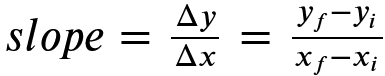
In this case y is Φ and x is t, so we have that:
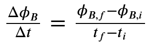
To translate this into code, we will need two different values for Φ. We can use the current value of Φ and the next value of Φ. This means that our initial value of Φ will be the value already calculated in line 41, the final value of Φ will be the equation for Φ evaluated at (t+dt), and the time step is simply dt. In the code this looks like:
deltaphi = (B*A*N*cos(omega*(t+dt)) - phi)/dtLine 43 – Instantaneous Change in Flux
To find the true instantaneous change in flux, we can take a derivative with respect to time of the flux equation:

In the code this becomes:
dphidt = -B*A*N*omega*sin(omega*t)Line 44 – Induced EMF
Faraday’s law tells us that the induced EMF is given by:
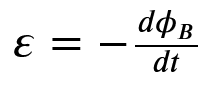
In the code we can simply put:
EMF = -dphidtPost-Coding Questions
- We could increase B, A, or ω. ω would be the easiest to increase because it would mean simply rotating the coil faster.
- To decrease the numerical error, we could decrease the value of dt.
- Initially the induced EMF is zero, then it is positive, and it switches direction whenever the coil and the B field are lined up.
- We assumed that the B-Field was constant.
Code
GlowScript 3.1 VPython
scene.range = 1.5

# Objects
coil = ring(pos=vector(0,0,0), axis=vector(0,1,0), radius=1, thickness=0.05,color = color.red)
wire1 = cylinder(pos=vector(-coil.radius,0,0),radius = coil.thickness,axis = vec(-50,0,0))
wire2 = cylinder(pos=vector(coil.radius,0,0),radius = coil.thickness,axis = vec(50,0,0))
Vindlabel = label(pos=vec(1.25,1,0), text='Induced EMF' )
Varrow = arrow(pos = vec(1.25,0.75,0),axis = vec(0,0,0),color = color.purple)

# Graph setup - ignore
Fluxgraph = graph(title='Flux and Change in Flux', xtitle='Time', fast=False, width=500)
f1 = gcurve(color=color.blue,  label = 'phi')
f2 = gcurve(color=color.orange,label = 'd phi/dt')
f3 = gcurve(color=color.black, label = "delta phi")
EMFgraph = graph(title='EMF vs t', xtitle='Time', ytitle = 'EMF [V]', fast=False, width=500)
f4 =  gcurve(color=color.red, label = "EMF")
Errorgraph = graph(title='Numerical Error', xtitle='Time',ytitle = 'Error', fast=False, width=500)
f5 = gcurve(color=color.blue,  label='Error')

# Setting up variables
omega = pi # in rad/s, this means the loop will rotate 180 degrees every second
B=1E-3  # T
A = pi*(coil.radius**2)
N = 500

#time setup
t=0
tf = 5
dt = 0.01

#Loop to make stuff happen
while t < tf:
  rate(100)
  coil.rotate(angle=(omega)*dt, axis=vector(1,0,0), origin=coil.pos)

  phi = B*A*N*cos(omega*t)
  deltaphi = (B*A*N*cos(omega*(t+dt)) - phi)/dt #approximate value
  dphidt = -B*A*N*omega*sin(omega*t) # true value
  EMF = -dphidt

  error = abs(dphidt-deltaphi)
  Varrow.axis = vec(0.1*EMF,0,0) #update the Vind arrow's size and direction (scaled down so the arrow isn't too big)
  f1.plot(t,phi)  # Plot everything
  f2.plot(t,dphidt)
  f3.plot(t,deltaphi)
  f4.plot(t,EMF)
  f5.plot(t,error)

  t = t + dt