Activity Information
Learning Goals
- Modify code to create a computational model of simple harmonic motion
- Understand how a net force causes a change in momentum
- Create graphs to analyze energy in a simple harmonic oscillator (HS-PS3-1)
Prior Knowledge Required
- Vectors
- Spring Force Equation
- The Momentum Principle
- Energy Equations
- Conservation of Energy
Code Manipulation
- Modify existing code
- Implement mathematical equations into code
Activity
Handout – Modeling Simple Harmonic Motion
All your hard work in learning physics has finally paid off—you’ve landed your
dream job at Hamerski Springs—a world leader in spring manufacturing and
consistently among the top 50 global companies based on a composite hipness
rating. And—giant bonus—you’ve been assigned to corporate headquarters in
Hanmer Springs, New Zealand!
Old man Hamerski has allowed his granddaughter to take over the tech division of the business. She was halfway through writing a computer simulation for simple harmonic motion of a mass oscillating on a spring when her best friend from Marahau asked her to help sail their family’s newly acquired 25-meter yacht, Zweisamkeit, up to the Marquesas Islands. In New Zealand, when your friend asks you to sail up to French Polynesia, the polite response is, “when are we leaving?”
So, the young Hamerski sends you a link to her code, wishes you good luck, and
promises a post card from Taioha’e. Your task is to finish the code such that it will be easy to change the mass of the oscillating object and the spring constant. The granddaughter likes to add plenty of comment lines to her code, so take advantage of that. Also, sketch out your plan so you can reference that while coding.
Code
GlowScript 2.9 VPython
scene.align = "left"
#The initial positions and specifications of the three objects are listed below.
#Make a sketch of these objects and label position coordinates.
#Remember, spring.pos is where one end of the spring is fixed, and spring.axis indicates the length and direction of your spring.
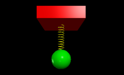
spring = helix(pos=vector(0,30,0), axis=vector(0,-20,0), coils=(10), radius=(3), thickness=(.5), color=color.yellow)
ball = sphere(pos=vector(0,0,0), radius=10, color=color.green, opacity=0.9)
support = box(pos=vector(0,35,0), size=vector(40,10,40), color=color.red)
#To get the system oscillating you will need some attributes defined.
#Below is the mass, spring constant, initial momentum of the ball, g, and energy values.
#Ug is gravitational potential energy. It is set to zero, but could be any value. Remember, we're really only concerned in how it will change.
#Us is spring potential energy. It is also set to zero. This is because it is neither stretched nor compressed. That will change as the ball moves.
#KE is kinetic energy. The ball is initially at rest, so it is zero to start. It will change as the velocity changes.
#ME is the total mechanical energy--simply the arithmetic sum of the other three energies.
mass = 5
k = 4
pball = vector(0,0,0)
g = vector(0,-9.8,0)
Ug = 0
Us = 0
KE = 0
ME = Ug + Us + KE
#The next 5 lines of code establish a graph that will plot the four energy values as the ball is oscillating up and down.
#The graph will be generated in the while loop below.
Grph1 = graph(title='Energy', xtitle='Time (s)', ytitle='Energy Values (J)', fast=False, align="right")
Grav = gcurve(color=color.red, label='Gravitational Potential')
Spri = gcurve(color=color.blue, label='Spring Potential')
Kine = gcurve(color=color.green, label='Kinetic Energy')
Tota = gcurve(color=color.yellow, label='Total Mechanical Energy')
#These 3 lines simply set the starting time to be zero, our tiny time increment to be 0.05 and the final time to be 15.
t = 0
dt = 0.05
tf = 15
#The "while" loop is where all the coding work is done.
#Both the spring force and gravitational force vectors are set at zero.
#You will need to write expressions for the calculation of each using what you know about the physics of those 2 forces.
#Each time the loop cycles, those forces will be updated. The updated forces are used to update the momentum of the ball.
#(remember, forces exerted for a little time increment cause a change in momentum)
#Once you update the momentum of the ball, you will need to update the ball.pos
#Then you will have to update the spring.axis because the spring needs to stay attached to the top of the ball.
#HINT: Every place you see a vec(0,0,0) you will have to change that to the correct physics expression to make the proper calculation.
#Similarly, all the zero energy values will need to be replaced with the proper formula using defined variables and/or numbers.
while t<tf:
rate(120)
sforce = vec(0,0,0)
gforce = vec(0,0,0)
fnet = sforce+gforce
pball = pball + vec(0,0,0)
ball.pos = ball.pos + vec(0,0,0)
spring.axis = spring.axis + vec(0,0,0)
Ug = 0
Us = 0
KE = 0
ME = Ug + Us + KE
Grav.plot(t,Ug)
Spri.plot(t,Us)
Kine.plot(t,KE)
Tota.plot(t,ME)
t = t + dtAnswer Key
Handout
Before doing the energy graphs, let’s get the motion of the ball and spring working. We know the spring force will be given by Fs = -ks, but we need to find what s is. Because the ball is starting at the origin, the displacement that it moves, which is the same as the stretch, will be given by its position. Translating this into code gives:
s = ball.pos.y
sforce = vec(0,-k*s,0)    # In the y-direction because the ball will move up and down
Now, we know the force from gravity equation is Fg = mg, so we can represent this in the code as:
gforce = mass*gThese added together gives us the net force. Multiplying this net force by a small time interval will give the change in momentum. In the code this looks like:
pball = pball + fnet*dtNow that the momentum is updated, the position needs to be updated as well. Multiplying the velocity by a small time interval will give the change in position. To get the velocity we can solve the momentum equation for velocity: p = mv => v=p/m. One way to implement this in the code is:
ball.pos = ball.pos + (pball/mass)*dt
spring.axis = spring.axis + (pball/mass)*dt  # The spring is attached to the ball, so the same velocity can be used to update its axis
Now the motion of the ball an spring should work. Lets sort out those energy graphs.
Near-Earth gravitational potential energy is given by GPE = mgh. However, we don’t know what h is, so we need to solve for it. This can be done with energy conservation. With the ball, spring, and Earth as our system, the total mechanical energy of the system will be conserved, which means that the energy at the top of the motion will be the same as at the bottom:
E(top) = E(bottom)
The ball starts from rest and has to stop for a moment at the bottom when it switches directions so the kinetic energy at each location is zero. At the top, the string isn’t stretched, so there is only GPE, and at the bottom the ball is at h=0 so there is only SPE:
E(top) = E(bottom) => mgh = 1/2ks^2
This looks like it still isn’t solvable, but s and h both represent the distance the ball moves, so we can say that s=h, which means we can now solve for h:
mgh = 1/2kh^2 => h = (2mg)/k
This is only the height when the ball is at the top of the motion, so to find the height at any point along the ball’s motion, we can take the difference between this value and the ball’s current position to find their separation vector. Implementing all of this in the code looks like:
Ug = mass*g.y*(((2*mass*g.y/k))-ball.pos.y)Spring potential energy is given by SPE = 1/2ks^2, which can be directly put into the code:
Us = 0.5*k*(s**2)Kinetic energy is given by KE = 1/2mv^2. Velocity is a vector, so to square it, we’ll need to take its magnitude. The code looks like:
KE = 0.5*mass*(mag(pball/mass)**2)Code
GlowScript 2.9 VPython

scene.align = "left"

#The initial positions and specifications of the three objects are listed below.
#Make a sketch of these objects and label position coordinates.
#Remember, spring.pos is where one end of the spring is fixed, and spring.axis indicates the length and direction of your spring.
spring = helix(pos=vector(0,30,0), axis=vector(0,-20,0), coils=(10), radius=(3), thickness=(.5), color=color.yellow)
ball = sphere(pos=vector(0,0,0), radius=10, color=color.green, opacity=0.9)
support = box(pos=vector(0,35,0), size=vector(40,10,40), color=color.red)

#To get the system oscillating you will need some attributes defined.
#Below is the mass, spring constant, initial momentum of the ball, g, and energy values.
#Ug is gravitational potential energy. It is set to zero, but could be any value. Remember, we're really only concerned in how it will change.
#Us is spring potential energy. It is also set to zero. This is because it is neither stretched nor compressed. That will change as the ball moves.
#KE is kinetic energy. The ball is initially at rest, so it is zero to start. It will change as the velocity changes.
#ME is the total mechanical energy--simply the arithmetic sum of the other three energies.
mass = 5
k = 4
pball = vector(0,0,0)
g = vector(0,-9.81,0)
Ug = 0
Us = 0
KE = 0
ME = Ug + Us + KE

#The next 5 lines of code establish a graph that will plot the four energy values as the ball is oscillating up and down.
#The graph will be generated in the while loop below.
Grph1 = graph(title='Energy', xtitle='Time (s)', ytitle='Energy Values (J)', fast=False, align="right")
Grav = gcurve(color=color.red, label='Gravitational Potential')
Spri = gcurve(color=color.blue, label='Spring Potential')
Kine = gcurve(color=color.green, label='Kinetic Energy')
Tota = gcurve(color=color.yellow, label='Total Mechanical Energy')

#These 3 lines simply set the starting time to be zero, our tiny time increment to be 0.05 and the final time to be 15.
t = 0
dt = 0.05
tf = 15

#The "while" loop is where all the coding work is done.
#Both the spring force and gravitational force vectors are set at zero.
#You will need to write expressions for the calculation of each using what you know about the physics of those 2 forces.
#Each time the loop cycles, those forces will be updated. The updated forces are used to update the momentum of the ball.
     #(remember, forces exerted for a little time increment cause a change in momentum)
#Once you update the momentum of the ball, you will need to update the ball.pos
#Then you will have to update the spring.axis because the spring needs to stay attached to the top of the ball.
#HINT: Every place you see a vec(0,0,0) you will have to change that to the correct physics expression to make the proper calculation.
#Similarly, all the zero energy values will need to be replaced with the proper formula using defined variables and/or numbers.

while t<tf:
    rate(120)
    s = ball.pos.y
    sforce = vec(0,-k*s,0)
    gforce = mass*g
    fnet = sforce+gforce
    pball = pball + fnet*dt
    ball.pos = ball.pos + (pball/mass)*dt
    spring.axis = spring.axis + (pball/mass)*dt
    Ug = mass*g.y*(((2*mass*g.y/k))-ball.pos.y)
    Us = 0.5*k*(s**2)
    KE = 0.5*mass*(mag(pball/mass)**2)
    ME = Ug + Us + KE
    Grav.plot(t,Ug)
    Spri.plot(t,Us)
    Kine.plot(t,KE)
    Tota.plot(t,ME)
    print(ball.pos.y)
    t = t + dt