Activity Information
Learning Goals
- Develop a computational model of the electric field from multiple point charges
- Understand how nested loops work
Prior Knowledge Required
- Vectors
- E-Field of a Point Charge
Code Manipulation
- Interpret Existing Code
- Create code from mathematical equations
Activity
Handout – Visualizing Electric Fields
Your school, Gnivri High, has decided to have a field day!
The catch is that instead of doing several track-and-field events, you and your team will be learning about fields in physics. Your team has decided to sign up for the electric field “event.”
Your team has been tasked with finishing this code that will show the electric field from point charges (click “remix” to save your own version). You’ve been given the following set of questions / instructions:
- Without Changning anything in the code, what happens when you run it?
- Read through the code and all the comments.
- What is the first set of loops (lines 20-34) doing collectively?
- What is each of these loops doing specifically?
- Hint: Try temporarily adding the code: rate(25) in line 25 to better see what is going on.
- Why are nested loops needed here?
- Draw a sketch of what you expect the E-Field to look like around particle1
- Change line 43 so it calculates the appropriate separation vector.
- Add an equation in line 44 that it calculates the appropriate Electric Field.
- Information found here might be useful
- How does your sketch compare to the E-field drawn by the computer?
- It would be much more interesting to see the E-Field from more than one point charge. Thankfully the code that you’ve just made will only need to be modified slightly to be able to do this.
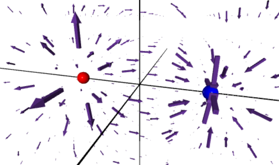
- Change particle1’s x position is -1.5 m.
- Add a second particle called particle2 that is identical to particle 1. Include it in plist.
- Change particle2’s x position to 1.5 m, its charge to -1, and its color to blue.
- Sketch again what you expect the E-Field to look like around and between these charges.
- Modify your code so that it calculates the E-Field at each observation point by adding up the field from both particle1 and particle2 at each point.
- Adding up the field from multiple sources is called superposition, and it’s very important in physics
- Hint: Use a nested for loop
- Try changing step in line 17 to 0.5. What do you observe now?
Code
GlowScript 2.7 VPython

#set the view - you might need to adjust this for your screen
scene.range = 3.5
scene.background = color.white

# Object setup
xaxis = cylinder(pos=vec(-7,0,0),axis=vec(14,0,0),radius = 0.01, color=color.black)
yaxis = cylinder(pos=vec(0,-5,0),axis=vec(0,10,0),radius = 0.01, color=color.black)
zaxis = cylinder(pos=vec(0,0,-5),axis=vec(0,0,10),radius = 0.01, color=color.black)
particle1 = sphere(pos = vec(0,0,0),radius = 0.15, color = color.red,q = 1)  # These are the point particles that are creating the E field
plist = [particle1] # Put the particle in a list - this will be much more useful when you add more particles

start = 3
obs = vec(-start,-start,-start) # Starting Observation location - where the first arrow will be placed
step = 0.75 # Spacing Between observer dots - change to 1 if the program is running slowly
obslist = [] # Initialize a list to store all of the observer arrows

#These loops create observer arrows in a 3d grid
while obs.x <= start:
  obs.y = -start        # Reset the y observer coordinate
  while obs.y <= start:
    obs.z = -start      # Reset the z observer coordinate
    while obs.z <= start:
      if obs.z == 0 and obs.y ==0: # This if statement omits observation points that are very close to the charges
        pass                       # so there won't be any gigantic field arrows
      else:
        testsphere = sphere(pos = obs,radius=0.005,color = color.black) # place a sphere at each observer location - this is just to make visualizing easier
        fieldarrow = arrow(pos = obs,axis = vec(0,0,0), color=color.purple) # Create an arrow with zero lenth at each observer location
      obslist.append(fieldarrow) # add all the arrows to obslist
      obs.z = obs.z + step # Increment the z observer location
    obs.y = obs.y + step   # Increment the y observer location
  obs.x = obs.x + step     # Increment the x observer location


# lets define some useful constants
k = 9e9        # Coulomb Constant
scale = 5e-11  # define a scaling constant to scale down the E field arrows
E = vec(0,0,0) # Initialize the E field

for arrow in obslist: # Loop through all the arrows
  E = vec(0,0,0)      # Reset the E field
  rsep = vec(0,0,0)


  arrow.axis = E*scale # Update each arrow's size and direction - scaled down so they aren't huge
Answer Key
Handout
- The program creates a set of axes, a red sphere at the origin, and a 3d grid of dots.
3. They are creating the 3d dot grid, as well as placing arrows of length 0 at each dot.
4. The first loop increases the locations of the observer dots in the x direction, the second loop does this in the y direction, and final loop does this in the z direction, and is the loop that actually places the dots and arrows.
5. We need nested loops because one loop would only create a single line of dots. We need a 2nd loop to get a 2d grid, and a 3rd loop to get a 3d grid.
6. Answers will vary, should show a point charge with arrows pointing away from it in all directions.
7. The separation vector is given by:
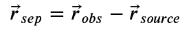
In this case, r obs is the position of an arrow and r source is the position of particle1. In the code this looks like:
rsep = arrow.pos - p.pos # Calculate the separation vector8. The equation for the E-Field from a point charge is:
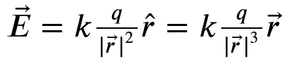
Translating this into code gives us:
E = (k*particle1.q*rsep)/mag(rsep)**3 # Calculate the E fieldIn the for loop this looks like:
for arrow in obslist: # Loop through all the arrows
  E = vec(0,0,0)      # Reset the E field
  rsep = arrow.pos - particle1.pos # Calculate the separation vector
  E = (k*particle1.q*rsep)/mag(rsep)**3 #  Calculate the E field


  arrow.axis = E*scale # Update each arrow's size and direction - scaled down so they aren't huge
9. Answers will vary.
10. This is as simple as changing the first entry in the position vector for particle1:
particle1 = sphere(pos = vec(-1.5,0,0),radius = 0.15, color = color.red,q = 1)11. This can be done easily by copying and pasting:
particle2 = sphere(pos = vec(-1.5,0,0),radius = 0.15, color = color.red,q = 1)
plist = [particle1,particle2]
12.
particle2 = sphere(pos = vec(1.5,0,0),radius = 0.15, color = color.blue,q = -1)13. Answers will vary, they should show arrows pointing away from the positive point charge and into the negative point charge.
14. This is the most difficult part of this problem because it requires creating a nested loop. The idea is that we can loop through each charge for each arrow, which means that we will need to create a for loop that loops over plist:
for arrow in obslist: # Loop through all the arrows
  E = vec(0,0,0)      # Reset the E field
  for p in plist:     # Loop through each charge
Here we could have used any variable we hadn’t defined already to represent the charges; I’ve elected to go with p. Within this loop we will need to include the separation vector and the E-Field equation. However, we will need to modify these to work with the new nested loop. Each charge is now represented by p, so anywhere that particle1 is called needs to be replaced with p:
rsep = arrow.pos - p.pos
E = (k*p.q*rsep)/mag(rsep)**3
We also need to make sure that we are adding up the E-field from each charge, so that equation needs to be changed to:
E = E + (k*p.q*rsep)/mag(rsep)**3This means that our final set of for loops looks like:
for arrow in obslist: # Loop through all the arrows
  E = vec(0,0,0)      # Reset the E field
  for p in plist:     # Loop through each charge
    rsep = arrow.pos - p.pos # Calculate the separation vector
    E = E + (k*p.q*rsep)/mag(rsep)**3 #  Calculate and add up the E field

  arrow.axis = E*scale # Update each arrow's size and direction
15. Decreasing step increases the number of observation points, and also moves some observation points closer to the charges. This means that the arrows near the charges get larger. In fact, the largest arrows pointing towards particle2 are so long that they appear to be pointing away from it.
Code
GlowScript 2.7 VPython

#set the view - you might need to adjust this for your screen
scene.range = 3.5
scene.background = color.white

# Object setup
xaxis = cylinder(pos=vec(-7,0,0),axis=vec(14,0,0),radius = 0.01, color=color.black)
yaxis = cylinder(pos=vec(0,-5,0),axis=vec(0,10,0),radius = 0.01, color=color.black)
zaxis = cylinder(pos=vec(0,0,-5),axis=vec(0,0,10),radius = 0.01, color=color.black)
particle1 = sphere(pos = vec(-1.5,0,0),radius = 0.15, color = color.red,q = 1)  # These are the point particles that are creating the E field
particle2 = sphere(pos = vec(1.5,0,0),radius = 0.15, color = color.blue,q = -1)
plist = [particle1, particle2] # Put both particles in a list

start = 3
obs = vec(-start,-start,-start) # Starting Observation location - where the first arrow will be placed
step = 0.75 # Spacing Between observer dots - change to 1 if the program is running slowly
obslist = [] # Initialize a list to store all of the observer arrows

#These loops create observer arrows in a 3d grid
while obs.x <= start:
  obs.y = -start        # Reset the y observer coordinate
  while obs.y <= start:
    obs.z = -start      # Reset the z observer coordinate
    while obs.z <= start:
      if obs.z == 0 and obs.y ==0: # This if statement omits observation points that are very close to the charges
        pass                       # so there won't be any gigantic field arrows
      else:
        testsphere = sphere(pos = obs,radius=0.005,color = color.black) # place a sphere at each observer location - this is just to make visualizing easier
        fieldarrow = arrow(pos = obs,axis = vec(0,0,0), color=color.purple) # Create an arrow with zero lenth at each observer location
      obslist.append(fieldarrow) # add all the arrows to obslist
      obs.z = obs.z + step # Increment the z observer location
    obs.y = obs.y + step   # Increment the y observer location
  obs.x = obs.x + step     # Increment the x observer location

# lets define some useful constants
k = 9e9        # Coulomb Constant
scale = 5e-11  # define a scaling constant to scale down the E field arrows
E = vec(0,0,0) # Initialize the E field

for arrow in obslist: # Loop through all the arrows
  E = vec(0,0,0)      # Reset the E field
  for p in plist:     # Loop through each charge
    rsep = arrow.pos - p.pos # Calculate the separation vector
    E = E + (k*p.q*rsep)/mag(rsep)**3 #  Calculate and add up the E field

  arrow.axis = E*scale # Update each arrow's size and direction